|
Week 1 - Week 2 - Week 3 - Week 4 - Week 5 - Week 6 - Week 7 - Week 8 - Week 9 - Week 10 - Week 11 - Week 12 - Week 13 - Week 14 - Week 15 - Week 16
Hope everyone's having a nice weekend and looking forward to Week 2. I'll try to get this up earlier in the week in the future, and for simplicity's sake, I'm going to try to streamline the flow as much as possible.
Every week, I'll summarize top five against-the-spread value plays and top five moneyline value plays. Both are based on teams' aggregate probabilities to cover or win across the 50+ NFL prediction models on The Prediction Tracker. I apply those probabilities to Westgate odds to produce expected values. I'll also post an updated summary of NFL futures values for all 32 NFL teams. In this case, I'm applying teams' average probabilities to win the division, conference, and Super Bowl across ESPN FPI, Football Outsiders, and Massey-Peabody Analytics to their Westgate futures odds to produce expected values. I am not suggesting that you bet these. In fact, the expected value of all of the futures below is negative. Good luck trying to win when the odds are literally stacked against you. Nevertheless, I find it interesting to see where the value potentially lies. (Please revisit Week 1 for more information about methodology.)
I. Against the Spread — Top 5 Value in Week 2
1. Tennessee +3.0 vs. Houston (even) — 70% chance to cover 2. Dallas -3.0 vs. N.Y. Giants (-110) — 62% chance to cover 3. New Orleans -9.5 vs. Cleveland (-110) — 59.3% chance to cover 4. Minnesota -0.0 at Green Bay (-110) — 59.2% chance to cover 5. Baltimore -0.0 at Cincinnati (-110) — 58.9% chance to cover For the second week in a row, the team playing the Houston Texans has the highest expected value against the spread, and the teams playing the N.Y. Giants and Cleveland Browns aren't far behind. That suggests that oddsmakers and the public like the Texans, Giants, and Browns more than the models do. That makes sense given that the models often look to last season as a baseline, when the Texans were injured, the Giants were bad, and the Browns were horrific. We'll see how things shake out in Week 2. Baltimore already lost at Cincinnati on Thursday night. Top five value plays were 4-1 in Week 1 (+390). LAST WEEK: 4-1 (+290) 65%+ COVERS: 2-0 (+200) 60%+ COVERS: 2-1-1 (+80)
II. Money Line — Top 5 Value in Week 2
1. Arizona: +750 at L.A. Rams — 23% chance to win 2. Tennessee: +145 vs. Houston — 62% chance to win 3. Buffalo: +280 vs. L.A. Chargers — 38% chance to win 4. Kansas City: +215 at Pittsburgh — 41% chance to win 5. Oakland: +240 at Denver — 38% chance to win These plays went 2-3 in Week 1, but because the list included underdogs (mostly heavy underdogs), that sub-.500 outcome would have generated meaningful profit. The Jets won as +250 underdogs at Detroit and the Bucs won as +375 underdogs at New Orleans. The Bears almost won (+260) at Green Bay, too. The plays listed here each week will almost certainly be underdogs. That's because the models think certain games are a bit more balanced than high moneyline odds imply. Check out Arizona for example. At +750, the odds suggest that the Cardinals have a 12% chance to win at the Rams, whereas the models suggest a 23% chance. A 23% chance to win $750 on a $100 wager equates to an expected return of $95.5. LAST WEEK: 2-3 (+325)
III. Searching for Value in NFL Futures Bets
When reviewing the table below, remember that the expected values listed are only as good as your faith in the probabilities that produce them. For example, if you think Washington really has a 3.0% chance to win the Super Bowl, then there is good value to be had at +5000 (50 to 1). But if you instead think Washington has a 2.0% chance at the Lombardi Trophy, you should view them as fairly priced at +5000. All this really does is compare the models' average probability of a certain event to the probability implied by Westgate's current odds. When the models' average probability is higher than the odds-implied probability, the expected value (or return on your wager) will be positive. There are very few such bets. Good value doesn't mean an event is likely. It just means you think it's more likely than the odds suggest. After last week's performance, the models believe the Jets have a 20% to win the AFC East, whereas New York's +1000 odds suggest a 9% chance. Value? Depends what you believe. Same logic for everything else. 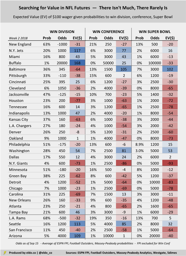
Note: Westgate did not have NFC North odds or a Vikings-Packers line as of September 15. I used 5dimes for those this week instead.

The primary data sources for this article were the Westgate Las Vegas SuperBook (odds as of September 15), ESPN Football Power Index, Football Outsiders, Massey-Peabody Analytics, and The Prediction Tracker. Data was compiled and analyzed by ELDORADO. All charts and graphics herein were created by ELDORADO.
The original version of this article framed expected value in terms of what a hypothetical $100 wager "would turn into." For example, if you were expected to lose $10, I showed the resulting expected value as $90, or $10 less than $100. I've since updated this to show the "expected return" on that $100 wager. So in that same example, the expected value now shows as negative $10. This is much more intuitive — positive expected values are good, and negative expected values are bad.
0 Comments
Week 1 - Week 2 - Week 3 - Week 4 - Week 5 - Week 6 - Week 7 - Week 8 - Week 9 - Week 10 - Week 11 - Week 12 - Week 13 - Week 14 - Week 15 - Week 16
With the Sunday of Week 1 upon us, attention has shifted from preseason futures to specific Week 1 wagers. But there's still a little more time to have some fun with those futures, so let's do that and then dive into Week 1. (Futures aren't going away, either — they just won't be preseason futures anymore.)
Some quick futures self promotion before we do. If you've ever wondered how preseason Super Bowl favorites fare, or where on the odds board Super Bowl winners typically come from, I wrote about that for FiveThirtyEight a couple of weeks ago. And if you've ever wondered about NFL win-total (over/under) trends — who trends over, who trends under, etc. — I wrote about that for ESPN a couple of days ago. Promos aside, I'm focusing on two topics in this article. First, I compare NFL futures odds to the probabilities published by three leading prediction models, and I use those odds and probabilities to show the expected value of a $100 wager on each NFL team to make the playoffs, win their division, win their conference, or win the Super Bowl. (I'll update this periodically over the course of the 2018 season.) Second, and along similar lines, I use aggregate game-by-game win and cover probabilities from 50+ NFL prediction models to calculate the expected value of a $100 wager on each NFL team to win or cover in Week 1. In the former case, the three prediction models are ESPN's Football Power Index (FPI)[1], Football Outsiders, and Massey-Peabody Analytics. In the latter case, the source is The Prediction Tracker.
--Here's an example of how this expected value stuff works. The New England Patriots are +600 to win the Super Bowl. That means that if a bettor wagers $100 on New England to win it all, s/he would win $600 if the Pats pull it off. But what's the probability of that actually happening? Heading into Week 1, the average probability of a Patriots championship across ESPN FPI, Football Outsiders, and Massey-Peabody is 14.1%.
In this example, our bettor has a 14.1% chance to win $600 and an 85.9% chance to lose $100. The expected value of betting $100 is therefore [14.1% x $600] minus [85.9% x $100], which equals negative $1.3. If you believe the probabilities offered up by the models, then betting the Patriots at +600 to win the Super Bowl does not provide good value. You're expected to lose a little bit of money if you do. The key is whether you actually believe the model-generated probabilities. If you thought the models were too bearish on the Patriots to win the Super Bowl and instead felt New England had a 20% chance, then +600 might look attractive to you. With a 20% chance to win it all, that same $100 bet has an expected value of [20% x $600] minus [80% x $100], which here equals +$40 — some potential value. I calculated the expected value of a $100 wager on every NFL team across four different futures bets — odds to make the NFL playoffs, win the division, win the conference, and win the Super Bowl: 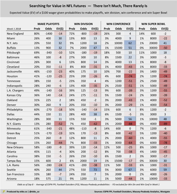
Futures are inherently unkind to bettors
The first thing to note is that the expected value of a $100 wager for almost every single one of these bets is negative. That tells (or reminds) us that futures are inherently unkind to bettors. The odds set by sportsbooks generally overstate the likelihood of each outcome, meaning futures bets carry heavy vigs.[2] There are literally only a handful of potential bets in each category that carry a positive expected return. And again, they hinge on whether you actually believe the probabilities that are put forth by the models.
Potential value bets — or not so fast
So where might there be some value? Well if you agree that Seattle has a 2.6% chance to win the Super Bowl — which the models suggest but most folks would consider too high — then there could be good value there at +6000 (60 to 1). And if you believe Washington really has a 1.47% chance to win it all, then they're undervalued at +10000 (100 to 1). Same for the Jets at 0.7% (200 to 1) and Tampa at 0.4% (3oo to 1). From a pure expected value perspective, most "potential value" comes by way of long shots like these, often because the models forecast higher probabilities for these teams than the public or oddsmakers believe.[3] The models also can't fully capture offseason sea (SEA?) changes, which is why Seattle looks so attractive. Remember to compare what you think to the models' probabilities listed in the table above. Pittsburgh is the only "good team" for which a Super Bowl futures wager currently carries positive expected value. That means the models like the Steelers a little better (10.7% to win it all) than the oddsmakers do (+1000, which has an implied probability of 9.1%). And if you agree that Baltimore has a 7.7% chance to win the AFC, or that Cincinnati has a 2.8% chance, there could be some light value there, too. Interestingly, if you agree that New England has "only" an 80% chance to make the playoffs — and thus a 20% chance to miss — betting the Patriots at +800 to miss the playoffs would carry better expected value than anything listed above. The expected value of that $100 wager would be +$80, or [20% x $800] minus [80% x $100]. The question again is whether you actually believe the probabilities. Brady injury, perhaps?
And what about the stay-aways?
From a conference championship and Super Bowl perspective, the math suggests that the Giants and Texans are greatly overvalued. The models give the Giants less than a 1% chance to win the NFC or the Super Bowl, making them a terrible bet at +2000 (20 to 1) or +4000 (40 to 1). In those cases, $100 wagers carry expected value of -$88 and -$89, respectively. Houston's expected values aren't much better. But whereas the models' inability to fully account for the offseason makes Seattle look like a better-than-reality bet, the same phenomenon makes the Giants and Texans look worse. New York drafted Saquon Barkley and is out from under Ben McAdoo, while Houston has Deshaun Watson and J.J. Watt back. Still, I'd argue that the odds for both teams get artificially compressed, making neither a great value play.[4]
Against the Spread — Top 5 Value in Week 1
1. New England: -6.0 vs. Houston (-110) — 66.4% chance to cover 2. Philadelphia: Pick 'em vs. Atlanta (-110) — 66.1% chance to cover 3. Pittsburgh: -4.0 at Cleveland (-110) — 62% chance to cover 4. Cincinnati: +2.5 at Indianapolis (-110) — 59% chance to cover 5. Jacksonville: -3.5 at N.Y. Giants (even) — 56% chance to cover The weekly "Coin vs. Machine" series I ran last season grouped picks into five tiers based on a handful of prediction models, and Tier 1 picks finished an impressive 35-22-2 (61.4%) against the spread. I won't be repeating that this year, but I will track the performance of teams with 65%+ or 60%+ chances to cover. Probabilities of covering come from an aggregate of 50+ models listed on The Prediction Tracker.
Money Line — Top 5 Value in Week 1
1. Chicago: +260 at Green Bay — 38% chance to win 2. Seattle: +130 at Denver — 54% chance to win 3 Tampa Bay: +375 at New Orleans — 24% chance to win 4. Buffalo: +275 at Baltimore — 29% chance to win 5. N.Y. Jets: +250 at Detroit — 31% chance to win The models to some degree reference last year's Packers, who went 7-9 without Aaron Rodgers for most of the season. That boosts Chicago's probability to win at Lambeau on Sunday. And as discussed earlier, the models don't quite know that Seattle is in a transition year, which artificially elevates their chances, too. Probabilities to win come from an aggregate of 50+ models listed on The Prediction Tracker. 
The original version of this article framed expected value in terms of what a hypothetical $100 wager "would turn into." For example, if you were expected to lose $10, I showed the resulting expected value as $90, or $10 less than $100. I've since updated this to show the "expected return" on that $100 wager. So in that same example, the expected value now shows as negative $10. This is much more intuitive — positive expected values are good, and negative expected values are bad.
Footnotes [1] ESPN's Football Power Index does not provide to-the-decimal probabilities for teams with less-than-one percent chances. (They're listed as <1%.) This affects five teams' probabilities to reach the Super Bowl and 11 teams' probabilities to win the Super Bowl. For purposes of this analysis, I coded these all as 0%, which is a conservative approach, but probably helps correct for some of the "reversion to the mean" inflation we see for bottom dwellers at the start of the season. [2] For example, if you were to add up the probabilities implied by each team's odds to win Super Bowl LIII, you'd find that they sum to 134.4%. Since 2001, the sum of all NFL teams' implied probabilities to win the Super Bowl has ranged from 126% to 158%. That's the result of overinflated odds, which essentially wrap the sportsbooks' profit into the futures odds. [3] Exact methodologies vary from model to model, of course, but there's often some use of last season's outcome as a reference point, overlaid with reversion toward the mean (downward for good teams, upward for bad teams), among many variables. Mean reversion can give teams at the bottom of the league better chances than they might actually deserve. [4] I don't have any scientific basis for this, but I suspect that Giants' odds get artificially bet down by Giants fans (e.g., the Giants should be 50/1 to win the Super Bowl but get bet down to 40/1.). Bill Simmons fans, for example, will recall hearing Cousin Sal joke about New Yorkers going to Vegas. And there are many. New York is by far the NFL's biggest natural market. (I say "natural" because many teams have fans beyond their regions, of course. The Cowboys' odds probably get compressed by the fact that they're "America's Team," for example. And yes, the Jets also play in NY/NJ. but they're the Jets.) I likewise suspect that Deshaun Watson's electric five-game run last season is pushing Houston's odds down, too.
The primary data sources for this article were the Westgate Las Vegas SuperBook (odds as of September 8), ESPN Football Power Index, Football Outsiders, Massey-Peabody Analytics, and The Prediction Tracker. Data was compiled and analyzed by ELDORADO. All charts and graphics herein were created by ELDORADO.
This story was updated on August 16, 2019 to reflect further improvements to the NFL wins pool draft order. The updated version is even more balanced. To skip down to the new 10-person draft order, click here. To skip down to similarly balanced draft orders for pools with nine, eight, seven, or six players, click here.
How to improve the "Bill Simmons draft order"
I was in my hometown a couple of weeks ago for an afternoon family event, so I floated a text to a couple of my buddies who live nearby to see what they were up to that night. As it turned out, a bunch of them were meeting at a bar a few hours later for their "fantasy football draft" — or at least what remained of it. After years on life support, their 14-year old fantasy league of 10 childhood friends — all dudes from the HS class of 2001, a year above me — had finally succumbed to the fact that we're in our mid-30s, most of the guys have little kids, and only Johan and Dan actually give a shit. (And Josh, but he'd never admit it.) So then what the hell were they doing there? And why show up at your friends' fantasy draft when they at least need to half-focus and having a couple of drinks / making fun of their picks / playing the role of court jester probably gets old by the draft's third round? My buddy McArdle's text revealed the answer: "We're doing a wins pool so the draft will be five minutes long. So you should come by if you're around." Ah. A wins pool. That sounds nice. The rules? Ten participants each pick three different NFL teams — using a unique draft order, which is the focus of this article — and whoever has the three with the most combined wins at the end of the regular season wins the pool. (The same team can't be picked twice.) Most importantly, wins pools require little or no preparation and zero time or attention during the season.[1] My own hometown fantasy league flirted with folding for five-ish years in a row too, each time inching closer to death, twice requiring that we grab a semi-random when one of the originals dropped out. We also ended up looking to a wins pool as a low-key way to keep some semblance of camaraderie alive.
The draft is easy — but the draft order is not entirely straightforward
If you sat down with nine friends to start a standard 10-person NFL wins pool, it wouldn't take long to realize that a traditional snake draft doesn't work — at least not fairly. Ten people making three picks across 30 NFL teams means three draft rounds, which is an odd number. Player 1 with the 1st overall pick would draft 1st, 20th, and 21st, while Player 10 with the 10th overall pick would draft 10th, 11th, and 30th. The sum of Player 1's draft positions is 41, and her average pick is 13.7. Meanwhile, Player 10's sum is 51, and his average is 16.7. There'd be a big advantage to picking early and big disadvantage to picking late.
The Bill Simmons draft order is fine — but we can do better
To remedy the snake draft issue — and extol the virtues of the wins pool upon America, which he's done successfully — Bill Simmons shared a wins pool drafting system on Grantland in 2012. Simmons did not create the draft order, but it has more or less become known as the "Bill Simmons draft order." Here it is: THE BILL SIMMONS METHOD Player 1 — 1, 20, 26 Player 2 — 2, 16, 29 Player 3 — 3, 13, 30 Player 4 — 4, 18, 25 Player 5 — 5, 15, 27 Player 6 — 6, 19, 22 Player 7 — 7, 11, 28 Player 8 — 8, 17, 21 Player 9 — 9, 14, 23 Player 10 — 10, 12, 24 Simmons concedes that he has "no idea how the creator came up with these numbers." But the order seems balanced enough — and in the end, NFL wins are random enough — that there isn't much reason to wonder. If you're curious, the Simmons wins pool draft order attempts to make the sum (or average) of each player's draft position as equal as possible. Every sum is 46 or 47, and every average is 15.3 or 15.7.
Last year was an improvement — but we can do even better than that
The "Simmons method" is better than the snake draft. But as originally detailed here in 2018, we were able to create a "fairer" wins-pool draft by basing the draft order on the sums and averages of historical win patterns, rather than the sums and averages of draft positions. It turns out that we can do even better. Down in the comments section, readers "Brian Golden" and "Harrison" suggested looking at how many games NFL teams typically win based on their preseason Vegas win-total lines. The idea is that when we all sit down for our NFL wins pool drafts, those win-total over/unders are the best market indication of how each team will perform, and that a logical wins pool draft order should therefore generally follow suit. Put another way, if wins pool drafts occur in descending order of preseason win-total lines — meaning the team with the highest win total gets picked 1st, the team with the 2nd-highest total gets picked 2nd, and so forth — then we could look back at how many games the team with the highest, 2nd-highest, 3rd-highest win totals (etc.) usually wins. A fair wins pool draft order should balance those projected wins. I was a little hesitant at first, in large part because I wasn't convinced that people actually drafted their wins-pool teams with win-total lines in mind. After all, there's only a modest correlation between preseason win-total over/unders and actual wins (0.46 since 2002). They tell us much more about how good a team was in the previous season (0.75) than do about how good they'll be in the upcoming season. But the comments stuck with me, so I decided to dive back in. I don't have look-through to hundreds or thousands of wins-pool draft results — if anyone does, let me know — but among the samples I analyzed, there was a 90% correlation between preseason win-total lines and wins-pool draft results. Consciously or not, people draft as preseason win totals suggest they should. Brian and Harrison's suggestion holds up.
How to improve your NFL wins pool draft order — balancing projected wins
Based on trends since 2002 — the start of the 32-team era in the NFL — the team with the highest preseason win-total over/under wins 12.3 regular-season games. The team with the 2nd-highest preseason win-total line wins 11.0 games, the #3 preseason team wins 10.2 games, and down from there. Overall, the top 30 NFL teams in terms of preseason win-total lines — the 30 that would be selected in a logical 10-person wins pool draft — go on to win 245.4 games. So to create a fair draft, we should structure the draft order so that each participant expects to win an average of 24.5 games across their three teams. Under the Simmons method, the person with the first overall pick (#1, #21, #26) has a major advantage. They project to garner 12.3 wins (#1), 6.9 wins (#21), and 6.6 wins (#26) — good for an expected total of 25.9 wins, or 1.4 wins above the equitable baseline. The person with the second overall pick (#2, #16, #19) also has a sizable advantage. In fact, every single player except Player #9 is at an advantage or a disadvantage. Anything can happen, of course, and these discrepancies aren't going to make or break your draft. But by reshuffling the deck based on the methodology described above, we can create an NFL wins pool draft order in which every player projects to win almost exactly 24.5 games. Here's how the revised order looks: 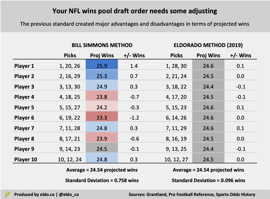
Due rounding, some numbers will not appear to sum
Under the new arrangement, all advantages and disadvantages are eliminated, and every participant's baseline is within 0.1 wins of the 24.5-win average. The standard deviation between the 10 wins-pool participants falls from 0.758 wins to 0.096 wins — a major decrease that greatly evens the playing field.
Here's a stand-alone summary with downward changes in red and upward changes in blue: THE ELDORADO METHOD Player 1 — 1, 28, 30 Player 2 — 2, 21, 24 Player 3 — 3, 18, 22 Player 4 — 4, 17, 20 Player 5 — 5, 15, 23 Player 6 — 6, 14, 26 Player 7 — 7, 11, 29 Player 8 — 8, 16, 19 Player 9 — 9, 13, 25 Player 10 — 10, 12, 27 I made it a point to still start the draft with a normal #1 through #10 order, making all of the changes elsewhere in the draft. There are other ways to arrive at a similar point — or perhaps to even flatten down the remaining 0.1-win discrepancies — but this order has produced the lowest standard deviation so far.[2]
The win-totals curve — and why Player 1's last two picks aren't as bad as they look
Although I feel confident that this method produces the fairest draft order yet, I worry that it might harbor some obstacles to adoption — specifically when it comes to the optics of Player 1's picks. After all, it looks pretty shitty to have the 1st pick but then not pick again until the end of the draft, in spots #28 and #30. But based on trends, the NFL team with the highest preseason win-total line projects to win 12.3 games, the team with the 28th-highest over/under projects to win 6.5 games, and the team with the 30th-highest over/under projects to win 5.9 games — good for a total of 24.6 wins between the three selected teams, which is essentially the spot-on projected average across all players. (It's actually a shade advantageous). Having the 28th and 30th picks isn't all that bad because preseason win-total lines aren't super accurate and the wins curve is really flat in certain areas. The 28th pick might sound bad on paper, but as you can see in the chart below, the actual wins it yields aren't much different from picking elsewhere in the 20s.[3] That's not the case at the very front end of the curve. There's a large premium to having the first overall pick — if you take the team with the highest win-total line, results are more consistent and you're reliably looking at double-digit wins. The best way to offset that is to also give Player #1 the 28th and 30th picks. In the following chart, you can see how many regular-season games NFL teams win (y-axis, out of 16 games) based on their preseason win-total over/under ranking (x-axis, out of 32 teams) before the season. 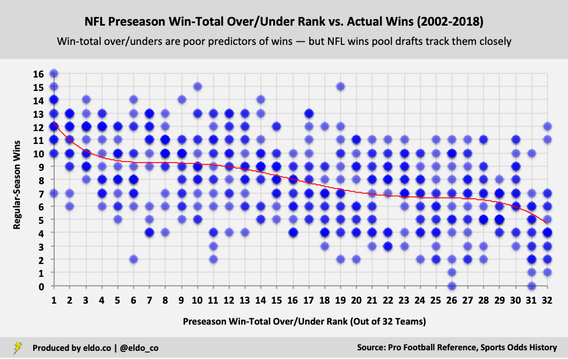
So when you've hit the point in your fantasy football league when a couple of people are auto-drafting, a couple more are forgetting to set their rosters, only two or three are working the waiver wire, and two or three more think that the guys who were good five years ago are still good (usually me), it could be time to hang your glory on the wall and switch to an NFL wins pool. Or just do one anyway because they're fun.
Don't have 10 players? — don't snake draft — these draft orders balance projected wins
NINE PLAYERS Player 1 — 1, 26, 27 Player 2 — 2, 18, 25 Player 3 — 3, 16, 21 Player 4 — 4, 14, 20 Player 5 — 5, 12, 23 Player 6 — 6, 11, 22 Player 7 — 7, 10, 24 Player 8 — 8, 15, 17 Player 9 — 9, 13, 19 Every player is within 0.1 projected wins of the average (25.2) except Player 1, who projects to win 25.4 games. But with the first overall pick and last two overall picks (#26, #27), this is the closest we can get Player #1 to the projected average. A traditional snake draft would only go back and forth 1.5 times, which is inherently unfair and does not account for the nuances of the wins curve. The revised draft order reduces the standard deviation from 0.8 to 0.1 projected wins. EIGHT PLAYERS Player 1 — 1, 17, 19, 32 Player 2 — 2, 16, 18, 31 Player 3 — 3, 13, 23, 29 Player 4 — 4, 12, 21, 28 Player 5 — 5, 10, 24, 25 Player 6 — 6, 9, 22, 26 Player 7 — 7, 11, 20, 27 Player 8 — 8, 14, 15, 30 Every player is within 0.06 projected wins of the average (31.9). A traditional eight-person snake draft would go back and forth two full times — which may be tempting — but because of the uneven win-projections curve, it would create a major advantage for Player #1 (0.8 projected wins above average), some advantage for Player #2 (0.2), and disadvantages for all others. The revised draft order reduces the standard deviation of projected wins from 0.33 to 0.04. SEVEN PLAYERS Player 1 — 1, 19. 20, 22 Player 2 — 2, 13, 21, 24 Player 3 — 3, 11, 18, 27 Player 4 — 4, 9, 17, 25 Player 5 — 5, 10, 15, 28 Player 6 — 6, 8, 16, 23 Player 7 — 7, 12, 14, 26 Every player is within 0.04 projected wins of the average (33.3). A traditional seven-person snake draft would also go back and forth twice, but because of the uneven win-projections curve — and the fact that spots #28-32 aren't there to offset the front end of the curve — it would create an enormous advantage for Player #1 (2.2 projected wins above average), a large advantage for Player #2 (1.0), and major disadvantages for all others. (If you snake draft with seven players, Player #1 starts with a 3.3 projected-win advantage over Player #7.) The revised draft order reduces the standard deviation of projected wins from 1.23 to 0.03. SIX PLAYERS Player 1 — 1, 12, 20, 23, 30 Player 2 — 2, 14, 16, 22, 26 Player 3 — 3, 11, 17, 19, 25 Player 4 — 4, 9, 13, 24, 27 Player 5 — 5, 7, 15, 18, 28 Player 6 — 6, 8, 10, 21, 29 Every player is within 0.02 projected wins of the average (40.9). A traditional six-person snake draft would only go back and forth 2.5 times here, which is inherently unfair and doesn't account for the nuances of the wins curve. The revised draft order reduces the standard deviation from 1.49 to 0.01 projected wins. In all of the scenarios above, I made it a point to give each player a first-round pick. In certain instances, you can reduce the remaining (negligible) imbalances even further if you don't hold yourself to that. I'm sure there are other ways to arrive at similar results. If you want me to run this for five, four, or three players, please comment down below! 
Footnotes
[1] The only instance I can think of in which an NFL wins pool might require some of your attention during the season would be if you were close to winning toward the end of the season and wanted to consider hedges. But that's optional. [2] If we had enough historical data, we could probably begin to factor in other variables, like how often the team with the highest win-total over/under is actually taken first (and so on and so forth), plus other variance in draft-order results and actual wins. Somebody out there could probably then use these probabilities and deviations to create an even fairer draft. [3] I suppose the same flatness and randomness argument could be spun back in defense of the Simmons method. As mentioned above, a few spots in something this random is not going to make or break your draft. But the goal here is to create the fairest draft possible with the data we have. And given the premium that exists for the player with the 1st overall pick, trends suggest that coupling the 1st pick with the 28th and 30th picks best balances and equalizes projected wins.
The main data sources for this article were pro-football-reference.com and sportsoddshistory.com. Data was compiled and analyzed by ELDORADO. All charts and graphics herein were created by ELDORADO.
HBO's reality sports documentary series Hard Knocks airs its third episode of the 2018 season on Tuesday night. Developed by HBO Sports and NFL Films and narrated by the legendary Liev Schreiber — whose mother bought him a motorcycle for his 16th birthday "to promote fearlessness" — the series follows one NFL team for a few weeks each August, offering behind-the-scenes access to the team's personalities and preparation. This year's featured team is the Cleveland Browns, who didn't win any games last season.
Hard Knocks debuted in 2001 and revolutionized sports-based reality television. But like so many good things, skeptics began to wonder what was the catch. Rumors of a Hard Knocks curse gained steam after the 2007 Kansas City Chiefs and 2008 Dallas Cowboys respectively suffered five- and four-game declines in their Hard Knocks seasons, the latter felled by a spate of injuries to Tony Romo and other starters. But whereas the Madden curse always felt ridiculous but believable in a fun and unscientific sort of way, the Hard Knocks curse really just felt ridiculous. One season after Dallas declined, the 2009 Cincinnati Bengals improved by six games and won the AFC North, and the season after that, the 2010 N.Y. Jets won 11 games and beat the Patriots in the Divisional Playoffs in Foxboro before losing in the AFC Championship. Nevertheless, the Hard Knocks effect still makes some waves each summer. And while there have been "myth of the Hard Knocks curse" articles out there for a few years, none has done more than quickly skip through team by team. So I decided to take a current and comprehensive look — consolidating the results, looking beyond just one season, and analyzing potential effects on the betting markets as well.
The 2001 Ravens were the first of 14 teams to go behind the Hard Knocks camera. The 2004 Jaguars technically appeared on an NFL Network series called Inside Training Camp: Jaguars Summer — the title of which beams of the same brilliance and creativity of Noah's Arcade (Wayne's World, anyone?) — but that edition is retroactively listed with Hard Knocks on NFL Game Pass and Hulu, so I am including it here.
Only five of the 13 teams (38%) who have completed their Hard Knocks season saw their win totals decline relative to the season before — the 2001 Ravens, 2007 Chiefs, 2008 Cowboys, 2016 Rams, and 2017 Buccaneers. While the average dip for those Hard Knocks squads has been a pretty substantial 3.6 games, the relative infrequency of decline is all you really need to know to dispel the Hard Knocks curse. Meanwhile, six Hard Knocks teams (46%) won more games in their Hard Knocks season than they did the year before, and two teams (15%), the 2002 Cowboys and 2015 Texans, equaled their prior season's win total. From 2009 through 2014, five straight Hard Knocks teams improved — ripe enough for a counter-narrative, perhaps, and yet the "Hard Knocks blessing" corner failed to gather any momentum at the time. Through 2017, Hard Knocks teams had a cumulative record of 102-105-1 in the season prior to appearing on the show, and they had a record of 100-108-0 in the season after — about as balanced as can be. 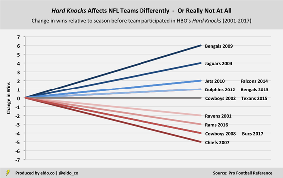
I also widened my analysis beyond teams' performance in the seasons immediately before and after Hard Knocks, looking as far as three seasons forward and three seasons back. When we look ahead and compare teams' incremental gains or losses in the win column relative to the season before they appeared in Hard Knocks, we see a continuation of the same trend as above — meaning no trend at all.
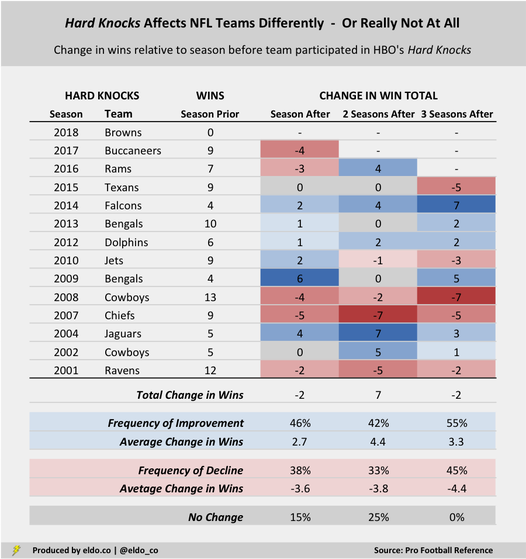
Two seasons after Hard Knocks, five out of 12 teams (42%) improved by an average of 4.4 games compared to their pre-Hard Knocks season; four of 12 (33%) declined by an average of 3.8 games; and three out of 12 teams (25%) were in the exact same position they were in before letting the cameras in. Three seasons after Hard Knocks, six out of 11 teams (55%) improved and five teams (45%) declined — a pretty even split.
If we really want to sniff out a trend, then perhaps we can argue that Hard Knocks teams were sort of on the rise before they appeared on the show, peaked the season after, and declined from there. The chart below captures the 11 Hard Knocks teams that participated through 2015; it excludes the 2016 Rams and 2017 Bucs because they don't have complete "seasons after" data. (And the 2018 Browns don't have any.) 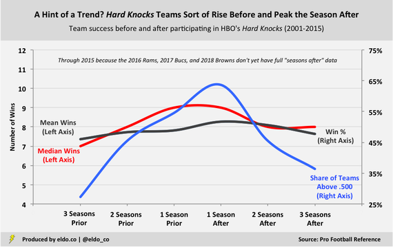
Three seasons prior to being featured, the average 2001 to 2015 Hard Knocks team had 7.4 wins and a 46.0% winning percentage. Only three out of the 11 teams were above .500 (27%). The season after appearing on the show, the average 2001 to 2015 Hard Knocks team had 8.3 wins and a 51.7% winning percentage, and seven out of 11 were above .500 (64%). That's the most trend-supportive stat in here.
But unfortunately for those in search of deeper meaning, these trends are muted by the (incomplete) addition of the 2016 Rams and 2017 Bucs. There's still a pre-Hard Knocks rise, of sorts, but the peak season becomes the season before the show, when the average Hard Knocks team wins 7.8 games.
While we're here, let's look at the relationship between Hard Knocks and the betting markets. Do Hard Knocks teams typically go over or under their Vegas win totals? Are their Super Bowl odds inflated or deflated by the fact that they're featured? Alas, as on the playing field, Hard Knocks is trend-less.
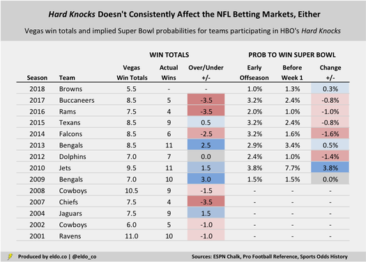
Seven of 13 Hard Knocks teams (54%) have gone under their Vegas win total in their Hard Knocks season by an average of 2.4 games; five (38%) have gone over by 1.8 games; and the 2012 Dolphins pushed. The 2017 Bucs. 2016 Rams, and 2014 Falcons were all noteworthy underperformers in recent seasons, but the 2013 Bengals, 2010 Jets, and 2009 Bengals punched the over in three of the four years prior to that.
Meanwhile, since 2009 — the earliest season for which I have Super Bowl odds from various points in the offseason — three out of nine Hard Knocks teams (33%) have seen their implied probability to win the Super Bowl increase after the show, five (55%) decreased, and one (11%) was unchanged. Rex Ryan and the 2010 Jets stand out for doubling their Super Bowl chances and delivering a very entertaining Hard Knocks. There is no Hard Knocks curse, and there is no Hard Knocks anything, really. Some teams go up, some go down, some go over, some go under, some improve in the eyes of the public, others decline. All we're left with is an entertaining series — and the "dulcet tones" of its fearless raconteur, Issac Liev Schreiber. 
The primary data source for this article was pro-football-reference.com. Data was compiled and analyzed by ELDORADO. All charts and graphics herein were created by ELDORADO.
Part I: France v Belgium - Part II: Time-Wasting Report Card
A few days ago, I wrote that France closed out Belgium with a master class in wasting time. I appreciate all the views it received and Twitter dialogue it's generated, much of which has seemingly come from the two countries involved in the match. Many great questions arose – namely how France's time-wasting in Tuesday's semifinal actually stacks up relative to other such performances in this World Cup and beyond.
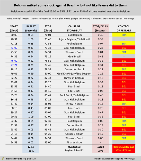
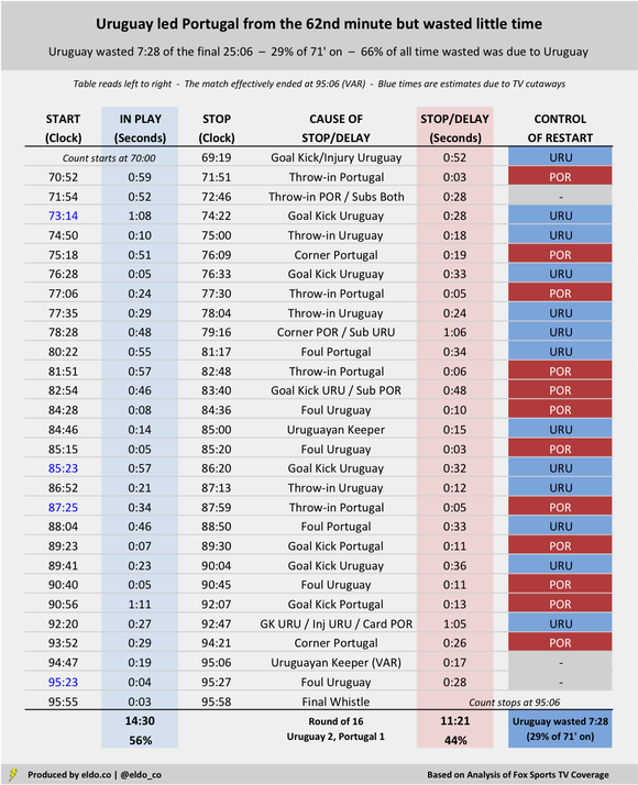
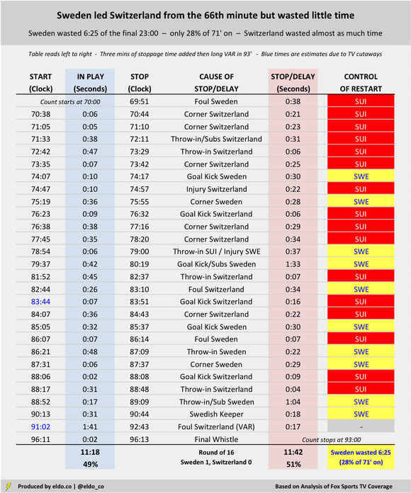
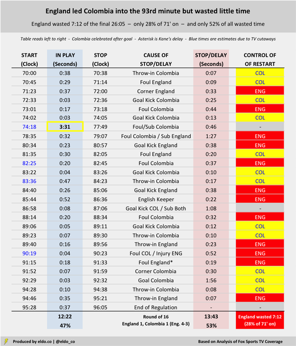
That is a question I absolutely wanted to explore, and I'd certainly have done it sooner if I could wave a magic wand and have the start-stop-and-cause data for every match at my fingertips. But in reality, it requires that I re-watch the end of every match. (Maybe there's some algorithm out there that can do it, though I'd argue you sometimes need human judgment to determine the primary cause of certain delays.) In any case, I went ahead and conducted the same "time-wasting" analysis for five additional matches from the 2018 FIFA World Cup knockout stage. I specifically focused on matches with a one-goal margin for all or nearly all of the 71st minute through the end of stoppage time, which mirrors the situation in France v. Belgium and is the most likely circumstance in which the side with the lead will waste time. So the sample now includes France v. Belgium (1-0, Semifinal); Brazil v. Mexico (2-0, Round of 16); Belgium v. Brazil (2-1, Quarterfinal); Uruguay v. Portugal (2-1, Round of 16); Sweden v. Switzerland (1-0, Round of 16); and England v. Colombia (1-1, Round of 16). Brazil had a one-goal lead from the 51st to the 88th minute, and England had a one-goal lead from the 57th minute to the 93rd minute, so both of those qualified. You can scroll down to see the play-by-play details for all six matches. The headline is that France did indeed waste time best (most) among World Cup teams with a one-goal lead in this year's knockout stage. Brazil was not far behind in their defeat of Mexico. Given the differences in stoppage time, the best measurement to lean on is percentage of the match after the 70th minute squandered by each side: 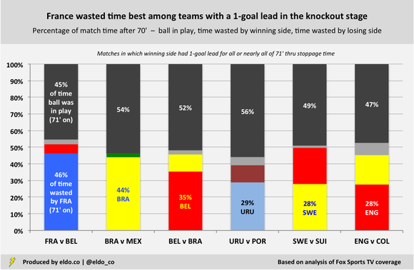
As we observed in the original story, France wasted 12 minutes and five seconds of the final 26 minutes and 13 seconds of their semifinal with Belgium, which represented 46% of all match time after the 70th minute. Brazil wasted 11:30 of the final 26:07 with Mexico, accounting for 44% of remaining time. Belgium milked some clock in their 2-1 quarterfinal victory too, but not nearly to the level of France and Brazil.
Brazil wasted time almost as well as France
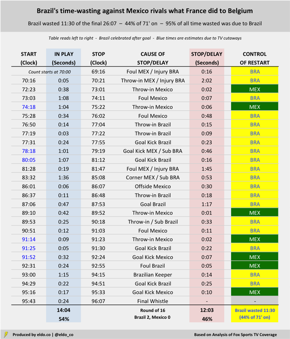
Brazil-Mexico's final stretch was an entertaining re-watch – depending, of course, on what your definition of entertaining is. I fast-forwarded as always to the 70:00 mark, and sure enough, play had already been interrupted by an injury to Brazil's Willian back at 69:16. The action didn't resume until 70:16. (For purposes of this analysis, I only counted the 16 seconds of stoppage that occurred from the 70:00 point onward.) Five seconds later (!!!!!), Neymar was writhing on the sideline in one of his finest performances of the World Cup. (I guess Miguel Layún stepped on him. You saw the GIFs and memes. You be the judge.) That resulted in a two-minute-and-two-second delay. Three-and-a-half minutes after that, he was back on the ground for a 48-second delay. Keeping track? That's 3:50 worth of Brazilian injuries in a span of 6:46. As if to one-up Neymar, Brazil's Thiago Silva took 1:45 off the clock with an injury that started at 81:47. Play resumed at 83:32, and for all his agony, Silva was back on the pitch 10 seconds later. In the period studied, Brazil burned 5:35 on injuries, 2:12 on subs, and 1:17 after a goal. That's 9:04 in wasted time after 69:17 alone. Surely there was more wasted in the half. Yet there were only six minutes of stoppage time. Four of Mexico's five fouls after the 70th minute sent a Brazilian player to the ground in histrionics. The only one that didn't came after Brazil secured a two-goal lead in the 88th. Yet somehow, when Brazil was trailing Belgium by a goal late in the next match, the Seleção avoided injury altogether. Brazil wasted only 2:34 after the 70th minute of that match – about one-fifth the amount they wasted against Mexico.
Everybody does it when they're winning (albeit to different degrees)
The winning side wasted more time than the losing side in all six of the knockout stage matches that carried a one-goal margin for all or nearly all of the end of regulation. France and Brazil fared comically best, followed by Belgium, and then Uruguay, Sweden and England. (England conceded a 93rd-minute goal to Colombia, so maybe they should have taken a time-wasting page from France and Brazil.) There's a ton of detail below, but I wanted to share it all because different folks will find different parts interesting. You'll note that winning teams were responsible for 71% of all time wasted after the 70th minute in these six matches. They were injured 11 times for a total of 13:59 (average of 1:16), whereas the trailing side was injured just once for a mere 22 seconds (Switzerland in the 75th minute against Sweden.) The winning side delayed the match with a sub nine times for a total of 8:53 (average of 0:59), while the losing team did so only twice for 1:19 (average of 0:39). (That doesn't mean losing sides didn't make subs after the 70th minute; it just means that when they did, there was another factor equal or greater causing the match delay.) Teams with the lead took twice as long on free kicks (31 seconds versus 15), and they took three times as long on goal kicks (31 seconds versus 11) and throw-ins (17 seconds versus six). [Again, the data below only counts the primary cause of delay. Injuries and substitutions generally take longer than whatever precipitated them, so they supersede the other acts listed. If a sub were made during a goal kick, for example, it's counted in the sub category, not as a goal kick. If an injury occurred to draw a free kick, it's counted in the injury category and won't show up in the free kick data. So for the most part, you can trust the corner, free kick, goal kick, and throw-in times as not elongated by other factors.] 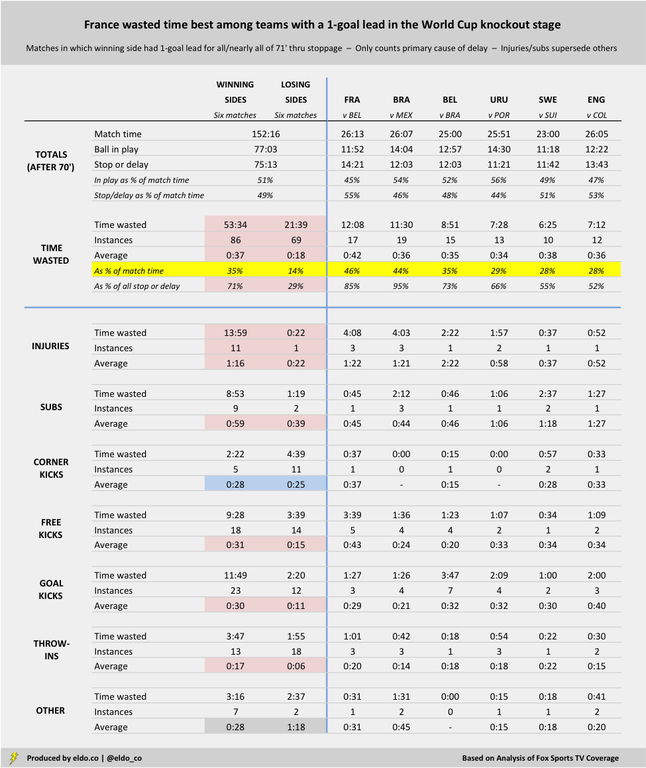
Detail for each of the six matches
Match flow can affect the degree to which a team has the opportunity to waste time. In the Round of 16, Switzerland trailed Sweden 1-0 from the 66th minute onward. But the Swiss maintained pressure and won six corners in the final 20 minutes plus stoppage time alone, losing 2:34 to a worthy but ultimately futile cause. (No other team in these six matches won more than two corners during that final run of the match.) The Swiss attack led to only two Swedish goal kicks, giving the Swedes less chance to burn clock. These charts are sorted by how much time the winning side wasted after the 70th minute. If you scroll all the way down to England v. Colombia, you'll see that I highlighted a continuous in-play stretch of three minutes and 31 seconds, from 74:18 to 77:39. That was by far the longest uninterrupted run of the periods studied in these six games. The next-highest was 1:41, during stoppage time of Sweden v. Switzerland. The average continuous play was 29 seconds – followed by, on average, 29 seconds of stoppage or delay. 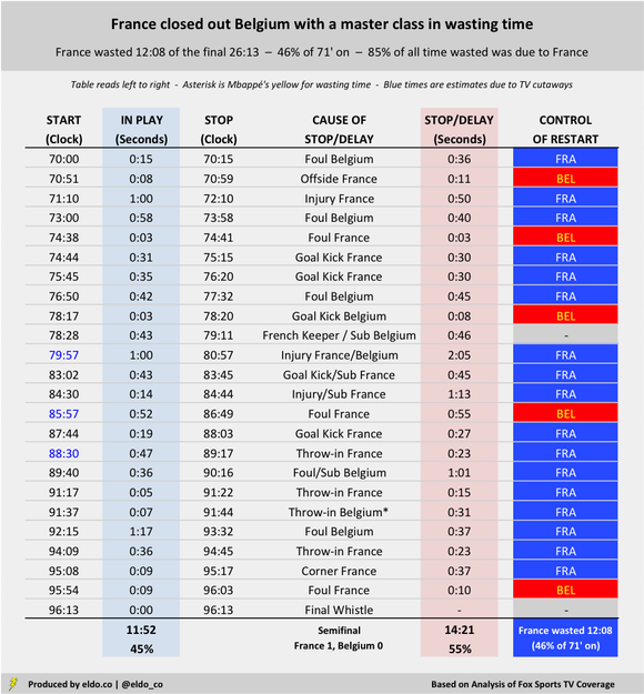

Times presented represent best estimates based on analysis of Fox Sports TV coverage. Three moments are asterisked because the camera cut away from the field. Other reasonable analyses might arrive at slightly different time estimates. Data was compiled and analyzed by ELDORADO. All charts and graphs herein were created by ELDORADO.
Part I: France v Belgium - Part II: Time-Wasting Report Card
France defeated Belgium 1-0 in the first World Cup semifinal on Tuesday, withstanding a few late pushes from The Red Devils with the help of two non-calls outside the box – and a master class in wasting time.
I reviewed the final 26 minutes of the match (70:00 through stoppage time) – during which France's time-wasting seemed to be most pronounced – and tracked starts and stoppages, their causes, and which team controlled each restart. Those final 26 minutes featured only 11 minutes and 52 seconds of action. You can see the details below. Keep in mind that FIFA considers certain stoppages like throw-ins and goal kicks to be "entirely natural," noting that a time allowance should be made only when delays are excessive. But at what point does "natural" for a goal kick or throw-in end and "unnatural" begin? FIFA separately instructs that injuries, substitutions, time-wasting, and celebrations should be factored into stoppage time.
French Goal Kicks (4) = 2 minutes and 12 seconds (71' on)
French Throw-Ins (3) = 1 minute and 1 second (71' on) France took four goal kicks during the final 26 minutes and shaved 30 seconds, 30 seconds, 45 seconds, and 27 seconds off the clock. (The third coincided with a French substitution). Their three late-match throw-ins burned 23 seconds, 15 seconds, and 23 seconds. Altogether, 3 minutes and 13 seconds of the final 26 minutes were paused for goal kicks and throw-ins – about one-eighth of the game's home stretch.
French Injuries (3) = 4 minutes and 8 seconds (71' on)
Injuries to France's Samuel Umtiti in the 73rd minute and Blaise Matuidi in the 81st and 85th minutes cost the match 50 seconds, 125 seconds, and 73 seconds, respectively – good for 4 minutes and 8 seconds in all. (Belgium's Eden Hazard was also hurt in the 81st minute, but he was back on his feet in 48 seconds..) When the whistle blew after Matuidi and Hazard's collision, the clock read 80:57. After play resumed, France milked a 45-second goal kick and substitute, Matuidi went down again, Belgium set up a long free kick, and France took another goal kick. The clock read 88:30. It was damn near the 90th minute, Over seven-and-a-half minutes had melted off the game clock. France and Belgium played for two of them.
French Free Kicks (5) = 3 minutes and 39 seconds (71' on)
Mbappé's Yellow = 31 seconds (92') France's Corner = 37 seconds (96') Les Bleus successfully squandered another 3 minutes and 39 seconds after five Belgian fouls (one of which led to a Belgian substitution); Kylian Mbappé took 31 seconds for his yellow-card inducing ball-bobbling antics in the 92nd minute; and France wasted 37 seconds before their 96th-minute corner. Six minutes of stoppage time were added. France and Belgium played for about two-and-a-half of them. From the 71st minute on (26 minutes and 13 seconds of match time), France and Belgium were paused or delayed for 14 minutes and 21 seconds – 55% of what should have been the most exciting part of the semifinal. France was primarily responsible for 12 minutes and 8 seconds (85%) of that wasted time.
I'm not saying all of that time should have been added back (though FiveThirtyEight found that World Cup stoppage time has been about half as long as it should be, even when you allow for the "natural" slippage associated with throw-ins and goal kicks). I don't even think you can really blame France. The rules are the rules, after all. Everybody wastes time when they're winning. France just did it extremely well today.
But it does kinda feel like FIFA needs to do something more. Howbout if you're down for one or two minutes you have to be substituted? Wouldn't that make these dudes get up? Actual increased stoppage time? Quicker yellows for modest delays? A red for something overt? I'm an American who only obsessively watches every four years, so I hold little authority. But I would love to hear your thoughts ; ) 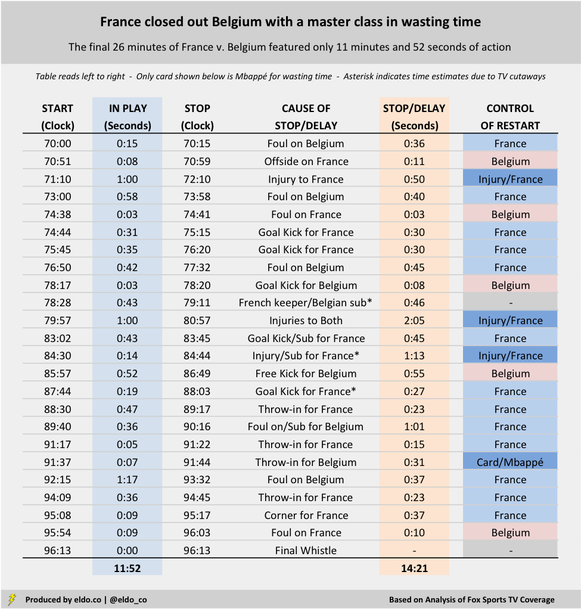

Times presented represent best estimates based on analysis of Fox Sports TV coverage. Three moments are asterisked because the camera cut away from the field. Other reasonable analyses might arrive at slightly different time estimates. Data was compiled and analyzed by ELDORADO. All charts and graphs herein were created by ELDORADO.
Spring 2018 officially came to an end last Thursday morning in the United States, and by the time the Fourth of July barbecues are fired up next week, the season that so reliably brings us flowers, baseball, and hay fever will be forgotten. As it turns out, there wasn't much "spring" to remember this year, anyway.
Spring spanned 94 days – March 20 to June 21 – but in New York City and surrounding areas (and many other places, I'm sure), it felt like it came late and left early. If forced elevator conversation is a reliable gauge of people's opinions on the weather, then you might recall strangers and coworkers complaining about how cold it was in mid-April, or how hot it was in early May. And if my own meandering observation is worth its salt, then I, too, felt robbed of that pleasant springtime stretch when it isn't too cold and it isn't too hot – when New Yorkers need not cover their faces from the bite of winter's cold or the sting of summer's stench. But were we really robbed? Did Mother Nature actually shortchange us of "spring"? Was there anything different or special about this past season?
I decided to test those casual observations and elevator conversations against data from the National Oceanic and Atmospheric Administration's National Centers for Environmental Information. I specifically focused on high temperatures in New York City's Central Park, and I took the liberty of defining "spring weather" as any day with a high in the 60s or 70s Fahrenheit. (That's 15.6 to 26.1 degrees Celsius.) From March 20 to June 21, New Yorkers experienced 40 days with a high of 60 to 79 degrees. That's the 10th-fewest "spring-weather" days since 1900. The other 54 days of spring were, of course, either colder (below 60) or hotter (80+) – decidedly "unspringlike" in the eyes of anyone who truly fancies the season.[1] 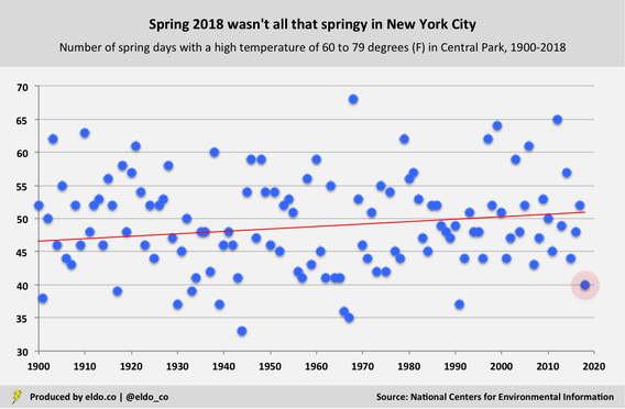
Another observation we can make is how many such days we had relative to how many we might expect. You may notice that the red trend line in the chart above tilts upward. In 1870, New Yorkers could expect about 45 days with highs in the 60s and 70s during the spring season. Rising temperatures have elevated that expectation to 51 days. In that way, today's New Yorkers generally enjoy the springiest springs of all. [The average high temperature for a spring day in Central Park has increased from 63.5 degrees Fahrenheit in the 1870s to 68.2 degrees this decade. I figured temperatures had risen but was surprised by the magnitude of the increase. That trend has reduced the number of sub-60 degree daily spring highs from approximately 36 to 24, and it's increased the number of 80-plus degree daily spring highs from 14 to 20.] Against that backdrop, our mere 40 spring days with highs of 60 to 79 degrees is even more noteworthy, as it's 11 days below expectation. That's the 8th-largest "below-expectation" recording since 1870, the first year for which complete data is available. It's also one of the few modern years on the list. In other words, not only was spring 2018 unspringlike, it was also far less springy than we've come to expect spring to be: 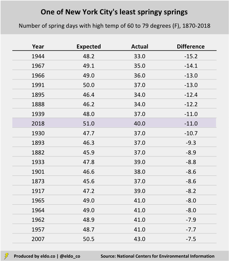
Average high temperatures tell a similar story. The average high this April was 57.1 degrees, which ranks in the 18th percentile for the month since 1900 – aka cold for April. The average high in May was 75.5, which ranks in the 93rd percentile for that month since 1900 – hot for May. That 18.4-degree difference between average highs in April and May is among the most drastic in recorded New York City weather history: 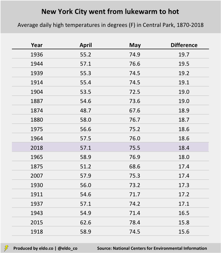
[If you walked into your office on April 19 with contempt for Mother Nature, you likely weren't alone. The high in Central Park that day was 49 degrees, or 15 degrees below normal.[2] During the first three weeks of April, high temperatures in New York City generally rise from 55 degrees (April 1) to 64 degrees (April 20); this year, highs were in the 40s on nine of those 20 days. And they were 51, 51, and 50 on three others.]
And what of summer, only a fews days young? So far, we're set to have our coldest June 21-to-26 stretch since 1992. The average high of 76 degrees over the six-day span is nearly six degrees below normal, and it's the city's 13th-coldest June 21-to-26 run since 1900.[3] So maybe spring lives on after all – until Friday, that is, when a four-day heat wave is expected to usher in highs of 90, 92, 94, and 92. Enjoy the summer! 
Footnotes & Extras
[1] To maintain a consistent baseline of comparison, I defined the spring season as March 20 to June 21 for all years. [2] From 1900 to 2018, the average high temperature in Central Park on April 19 was 63.7 degrees Fahrenheit. [3] From 1900 to 2018, the average high temperature in Central Park from June 21 to 26 was 81.8 degrees Fahrenheit. 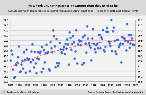
The source for this article was the National Oceanic and Atmospheric Administration's National Centers for Environmental Information. Data was compiled and analyzed by ELDORADO. All charts and graphics herein were created by ELDORADO.
Earlier this week, the Supreme Court struck down a 1992 federal law that effectively prohibited sports betting in the United States, save for a handful of state-specific exceptions. In a 6-3 decision, the court ruled that the Professional and Amateur Sports Protection Act (PASPA) violated the 10th Amendment, which limits the federal government from controlling state policy.
The decision paves the way for states to decide whether to offer legal sports betting. ESPN’s David Purdum reports that New Jersey, which brought the case, Mississippi, New York, Pennsylvania, and West Virginia could be among the first to do so. The Associated Press reports that as many as 14 states could act within the next two years, with another 18 states to follow. So what does the decision mean for you? For starters, it’s likely to bring much of the estimated $150 billion-dollar-a-year black market in sports gambling above board.[1] You’ll conceivably be able to place a bet on your phone, at a local sportsbook, or even in an arena. Casinos should see a boost. And fans will have more reason to engage, which supports broadcasters, franchises, and leagues. Most importantly, however, the Supreme Court’s decision on sports betting means that you will now be able to lose your money legally – which, either right away or over time, you are exceedingly likely to do.
At the start of last NFL season, I walked through some of the success rates and financial dynamics of the most popular sports wager in the United States – the spread bet. I specifically looked at the against-the-spread performance of 60 individuals and 60 prediction models during the 2016 NFL season. I’ve since updated those statistics to include the 2017 NFL season.
To the unfamiliar, here’s an example of how a spread bet works. Assume the Dallas Cowboys are 4.5-point favorites at home against the New York Giants. If you pick Dallas to win “against the spread,” they need to win by five points or more for you to win the bet (“Dallas -4.5”). If you pick New York, you win if the Giants win the game outright or lose by four points or less (“Giants +4.5”). In a typical spread bet, you risk 10% more money than you would win (-110), known as a 10% “vig.” Bet $110 and win, and you get $100. Bet $110 and lose, and you lose all $110. Historically, sportsbooks would set and adjust point spreads to attract and maintain equal action on both teams.[2] Doing so guarantees the books a profit on those bets, equal to 4.5% of the total amount wagered.
The chart below shows the results of a random group of individual bettors (60 in 2016 and 53 in 2017) and prediction models (60 in 2016 and 57 in 2017) “against the spread” over the course of the last two NFL regular seasons. As expected, both groups had an average success rate right around 50%. And while the sample size is still small, you can see a typical bell curve forming.
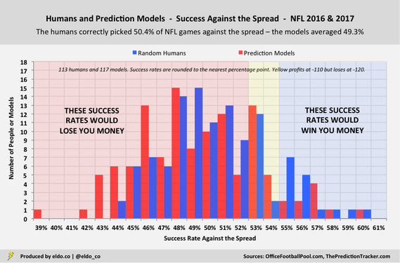
Half of the bettors won more games than they lost, and half lost more games than they won. But when losses cost $110 and wins only earn $100 – thanks to that 10% vig – things get pretty ugly pretty fast. Had everyone wagered real money on every game in equal amounts, only 30 out of 113 individuals (27%) would have netted a single-season profit. Nearly three-quarters of bettors would have lost money.[3]
Now consider this. Certain professional sports leagues have been lobbying to receive an “integrity fee” for all wagers placed on their respective games, theoretically compensating them for “[creating] the source of the activity” and “[bearing] the majority of the integrity risk.” Fee estimates range from 0.25% to 1.0% of money wagered, or 2.5% of profits, with other wrinkles attached. Sports betting operators will also have to pay taxes – potentially as high as 12.5% of gross sports wagering revenue in one version of an Illinois bill. Against this backdrop, rumors began to circulate last fall that sportsbooks might consider covering these taxes and fees by raising the standard vig from 10% (-110, risk $110 to win $100) to 20% (-120, risk $120 to win $100). If that happens, your chances of making money get even dimmer. With a 10% vig in the example above, we saw how roughly three out of four individual bettors would have lost money – already pretty tough sledding. With a 20% vig in the same example, nearly seven out of eight would have lost money on a single-season basis – worse still, 95% of the individuals who were part of the sample in both years would have lost money over the course of the two seasons combined.[4]
Let's take a closer look at just how devastating the vig is. With a 10% vig, only three out of 113 individuals (2.7%) would have netted a single-season return-on-dollars-wagered of 10% or more. Meanwhile, 22 people (19.5%) would have had a 10%+ loss. Only 18 of the individuals would have earned a 3%+ profit, while 61 bettors would have lost at least that much. And the 20 worst performers would have lost over 2.0x the money that the 20 best performers gained.
Now let’s repeat those sentences assuming a 20% vig. With a 20% vig, only one out of 113 individuals (0.9%) would have netted a single-season return-on-dollars-wagered of 10% of more. Meanwhile, 50 people!!! (44.2%) would have had a 10%+ loss. Only four of the individuals would have earned a 3%+ profit, while 83 bettors would have lost at least that much. And the 20 worst performers would have lost almost 8.0x the money that the 20 best performers gained. And again, those are single-season returns. It's even harder to stay in the black year over year. With a 10% vig, bettors in this example would have had to finish in the 90th percentile in 2017 just to offset the damage of finishing in 50th percentile (i.e., being exactly average) the year before. (Remember that half of the bettors did even worse!) With a 20% vig, they'd have had to finish in the 97th percentile in 2017 to recoup the money they lost by finishing in the 65th percentile (above average!) the year before. In other words, the reward for being good-but-not-great is a financial penalty and a requirement that you be exceptional next year to break even. You can deduce from the chart how ugly it gets when you're actually below average, like half of everybody is. 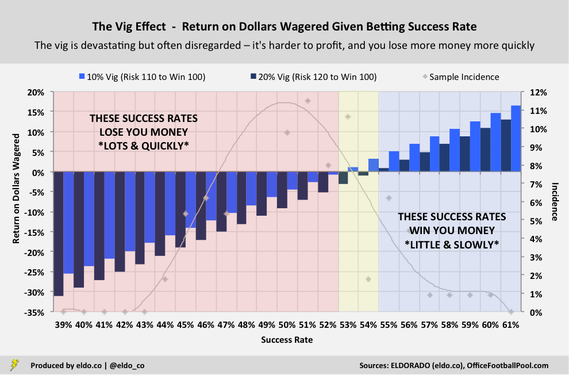
Despite all that, most folks kinda pretend the vig isn’t there, casually chalking it up as the cost of doing business. Ask your buddy how much he has on a game, and he’ll likely say “$100” or $50,” not “$110” or “$55,” which is really what he’d lose. If he wins two bets and loses two others, he’ll probably tell you that he went two and two, not that he lost money.
Of course, not everyone puts money on every game. Bettors often target select games. But even then, one person's "best bet" is another's "trap of the week," and over a long enough period, the vast majority of casual bettors will lose money. There’s nothing special about the math. Sometimes we just need to see it all on paper. 
Footnotes
[1] Market estimates vary wildly, from $67 billion to $380 billion. For context, Nevada sportsbooks handled $4.8 billion in sports wagers in 2017. [2] Evidence suggests that sportsbooks have grown increasingly comfortable straying from that 50-50, guaranteed-profit balance. When they do so – that is, when they set lines that attract significantly more money on one team – they’re effectively betting on the other team. In early 2017, certain books allowed big imbalances in nine of 10 NFL playoff games. The books lost all of them against the spread. [3] In this particular sample, that's true both on a single-season basis and combined over the course of the two seasons. There were 60 individuals in 2016 and 53 individuals in 2017. Forty-two of them were the same across seasons. On a single-season basis, 83 out of 113 (73%) would have lost money with a 10% vig. On a combined basis over the two seasons, 31 out of 42 (74%) would have lost money with a 10% vig. [4] Again, there were 60 individuals in 2016 and 53 individuals in 2017. Forty-two of them were the same across seasons. On a single-season basis, 97 out of 113 (86%) would have lost money with a 20% vig. On a combined basis over the two seasons, 40 out of 42 (95%) would have lost money with a 20% vig. Portions of this story were updated and adapted from one of my previous posts.
Data was compiled and analyzed by ELDORADO. All charts and graphics herein were created by ELDORADO.
(And other musings on the history, controversy, irony, stereotypes, cultural associations, and cultural complexity that the show and its cast have brought to light)
MTV’s Jersey Shore: Family Vacation airs its seventh episode on Thursday, and the reunion season has managed to reinsert the likes of Deena, JWoww, Pauly D, Ronnie, Snooki, The Situation, and Vinny back into certain corners of pop culture. (Sammi Sweetheart isn’t even there and yet she’s kinda back, too.) Technically a new series – and already renewed for a second season – episodes have drawn between 1.44 and 2.55 million viewers, making it the highest-rated original cable show among 18-to-49 year-olds on all but two of the Thursday nights it’s aired. The only telecasts that topped it were the NFL Draft on April 26 and the NBA Playoffs on May 3.[1] While strong, those numbers are a far cry from Jersey Shore’s original six-season run, which spanned 71 episodes over three years and peaked at 8 million-plus viewers per episode. At its apex, it was the second-most watched Thursday-night show on cable or network television for 18-to-49 year-olds, behind only American Idol on Fox. 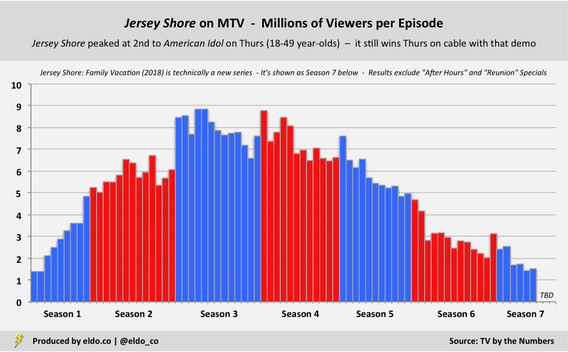
The fact that Jersey Shore still commands attention and dominates its night on cable – nearly a decade after its premiere – is a testament to how much of a pop culture juggernaut it was. The show that gave us GTL, T-shirt time, and "the note" successfully brought contemporary guido culture to the mainstream. Its popularity surged despite controversy – or perhaps because of it – and in spite of another interesting and telling cultural fact, the significance of which extends far beyond Thursday nights on MTV.
Jersey Shore’s cast members are self-proclaimed “guidos” and “guidettes,” and MTV originally ran promos declaring that they’d brought together the “hottest, tannest, craziest guidos” for the show. The program’s negative portrayal of Italian-Americans ignited criticism from several Italian-American organizations, and MTV’s use of the pejorative “guido” in promos prompted Domino’s Pizza to withdraw as an advertiser. (Ten more national advertisers followed suit. MTV removed the word from promos and descriptions but let it run free in the show.)
Every American ethnic group has its stereotypes. But with Jersey Shore, we have a show built around people who actively associate their idiocy, however mindlessly entertaining, with the negative stereotypes of one particular group. The cast flies the proverbial flag – or paints it on their chests – and advances, explains, and justifies their antics as “Italian-American.” Worse yet, if you actually lift up the genealogical hood, you find that the Jersey Shore cast is barely over half Italian-American: 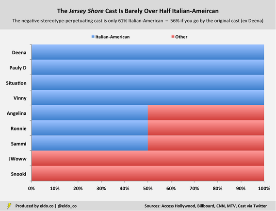
Only three of Jersey Shore’s eight original cast members claim full Italian ancestry – Paul DelVecchio ("Pauly D"), Mike Sorrentino ("The Situation"), and Vinny Guadagnino. Three others, Angelina Pivarnick, Ronnie Ortiz-Magro, and Sammi Giancola ("Sammi Sweetheart"), are half Italian-American. (Angelina is Polish on her father’s side, Ronnie is Puerto Rican on his mother’s side, and Sammi is Greek on her mother’s side.) Jenny Farley ("JWoww") and Nicole Polizzi ("Snooki") do not have any Italian ancestry at all.[2]
What we end up with is the bastardization of a culture by a group of people who, to a sizable extent, merely chose to represent it. And there’s an interesting irony to that. For generations, many Italian-Americans (and members of other immigrant groups) felt compelled, thought it an advantage, or otherwise elected to Americanize their names and whitewash their Italian ancestry, which American society viewed as somewhere between "too ethnic" and "criminal." (Sound familiar?) Some were stars. Others might have been your parents or grandparents.
In 1963, Anna Maria Louisa Italiano from the Bronx won the Academy Award for Best Actress for The Miracle Worker. America knew her as Anne Bancroft. Dean Martin was born Dino Paul Crocetti in Steubenville, Ohio. Tony Bennett is Anthony Dominick Benedetto from Queens. In 1972, six out of 13 Italian-American congressmen “had either English or Americanized family names.” Whoever signed up my mother’s Italian-immigrant father for school in the Bronx took the liberty of making a similar first- and last-name switch for him. And still harboring this old-school mindset in the 1990s, my father’s father once politely told me to consider changing my own name if I wanted to pursue certain public professions. As recently as 1983, The New York Times Magazine ran a long piece on “Italian-Americans Coming into Their Own,” highlighting that “Americans of Italian descent… [had] attained a kind of critical mass in terms of affluence, education, aspiration and self-acceptance.” The article opens in the offices of three-term New York Governor Mario Cuomo and offers a fascinating glimpse into how the Italian-American journey was felt and perceived at the time. It closes with the story of William D'Antonio visiting his daughter Laura at college. Laura comments that she's "the only 100% Italian in [her] dorm... but [she knows] at least a dozen people who wish they were Italian." William muses that 40 years earlier, "[he] would not have been able to admit that [he] was Italian, much less imagine any dozen people who wished they were.'' Progress had come. And so far gone are the days of Italian-Americans changing their names that today's performers and politicians not only keep them, some voluntarily adopt them for art or appeal. When New York City hosted the 60th Annual Grammy Awards in 2018, headline acts included Alessia Cara, Italian-Canadian; Stefani Joanne Angelina Germanotta, three-quarters Italian and better known as Lady Gaga; Donald Glover, who raps under the stage name Childish Gambino; and Logic, whose mixtape titles bear the names of Sinatra and Tarantino. Even the host city’s mayor, Bill de Blasio, opted into an Italian name – he was Warren Wilhelm until 1983 and Warren de Blasio-Wilhelm until 2001. We’re a long way from Anne Bancroft, Dean Martin, Tony Bennett, and my grandparents’ generation.
But the Jersey Shore phenomenon still underscores a major cultural paradox. Many Italian-Americans don’t carry the hyperbolic physical or behavioral hallmarks that American society perceives to mean “Italian-American.” So when Italian-Americans are successful, that success is not closely associated with their ethnic or family background. If you walked into a room and chatted with Geraldine Ferraro (the first female vice-presidential candidate of a major U.S. political party), Samuel Alito (the 110th Justice of the Supreme Court), or Anthony Fauci (pioneering HIV/AIDS researcher and Director of the National Institute of Allergy and Infectious Diseases since 1984), would you walk out thinking they were all Italian-American? Unless you saw their names or discussed the topic of family origin, you might believe none of them was.
[It’s scary to wonder how many more people know who Snooki is than Geraldine Ferraro.] Conversely, if you walked into a room and chatted with a bunch of Jersey Shore-style personalities, you’d likely walk out thinking of them as uniformly Italian-American – even though the Jersey Shore cast, the wannabe guidos at your New York-area high school, and the lines outside of Neptunes in the Hamptons (R.I.P.) and D’Jais in Belmar might be about half, if even that. Everyone else is opting in, flying the flag, painting it on their chest – either halfway or all the way. [If you’re tempted to comment that those people and places are “more Italian-American than I think,” you’re only proving my point.] And yet that image gets projected out into the world, so much so that respectable media organizations feel comfortable running Anthony Scaramucci headlines like “Donald Trump has gone full Sopranos with his latest hire,” “Reince Priebus sleeps with the fishes,” and “A Scaramucci-watchers guide to Italian-American speech” – to little criticism, I might add, even though we live in a Twitterverse where every perceived ethnic slight is harshly and immediately punished. Stephen Colbert played the mafia card, too. As Joan Vennochi wrote in a similarly titled but very thoughtful Boston Globe story, “when it comes to making fun of other ethnic groups, politically correct limits usually apply. No such restrictions govern parodies about Italian-Americans. The tribe itself is torn by ambivalence over its portrayal.”
It took Italian-Americans a generation to learn the language and a couple more to “make it” in America. But in the end, we are fortunate to have earned[3] – and eventually been permitted to earn – our slice of the American Dream, even with the early poverty and violence, the National Origins Act and No Italians Need Apply, and today’s still-too-common guido stereotypes and mafia portrayals along the way.
My goal here is to offer perspective and gratitude, not complaints. After all, a little Jersey Shore bullshit is more nuisance for Italian-Americans than actual threat, which is what many other groups still face. Our threat days are over. So now it's time for that perspective and gratitude to extend beyond our own dinner tables – to support other groups who harbor the same multi-generational American hope, to those who were never given their fair shake in this country, and to those who pursue the Dream today. 
Footnotes
[1] For added context, Jersey Shore: Family Vacation has drawn 2.2 to 3.3 times the total viewers per episode as FX's critically acclaimed Atlanta and 1.3 to 1.5 times the total viewers per episode as Bravo's popular Southern Charm. All three air on Thursday nights. [2] Deena Cortese replaced Angelina after season two and is Italian-American on both sides of her family. JWoww is Irish- and Spanish-American. Snooki is Chilean-American but was adopted and raised by an Italian-American family. In a 2010 interview with Fox News, JWoww pointed out that she and Snooki are not Italian-American and that they're "not trying to be Italians." For what it's worth, it feels a little weird to analyze people’s ethnic backgrounds like this, but if the Jersey Shore cast wants to represent Italian-American culture – or at the very least if they're going to be universally associated with it – it's only proper for the rest of us to check the facts. [3] The real hard work and sacrifice came in the generations before me. I am forever grateful for that.
Data was compiled and analyzed by ELDORADO. All charts and graphics herein were created by ELDORADO.
Best QB Draft Classes in History | QB Draft Class Facts & Figures
The sister post to this one covers the best quarterback draft classes in NFL history in terms of era-adjusted passing yards. For more on those legendary classes, please check out the original story.
Developing that story kicked up a lot of other fun facts – including the number of active QB draft classes in the league in a given season, draft-class longevity, draft-class peaks, the worst draft classes in NFL history, and, more generally, the best quarterback seasons and careers based on our era adjustment. The facts laid out below come from my analysis of Pro-Football-Reference.com data.
The Number of Active QB Draft Classes
- Quarterbacks from 18 different draft classes recorded passing statistics during the 2017 season, tying the 2004, 2003, 1975, and 1969 seasons for the most in NFL history. Of those, 2017 is the only one in which the 18 draft classes were consecutive (2000 through 2017). All of the others had gaps – 2004 and 2003 because of Doug Flutie's longevity (QB Class of ’85) and 1975 and 1969 because of George Blanda's (’49). - There have been between 14 and 18 QB draft classes active in every NFL season since 1961. The average over that period (and post AFL-NFL merger) is 15.75. The seasons with 18 active QB classes were mentioned above. Interestingly, the seasons with 14 active QB classes have all come in twos or threes – 2013 and 2012; 1992 and 1991; 1986, 1985, and 1984; 1981 and 1980; and 1962 and 1961 – and are generally due to a lack of longevity among what, in those seasons, should've been the elder quarterback classes. - The older end of the 2017 season's draft-class curve was made up of Tom Brady (2000), Drew Brees (2001), Josh McCown (2002), and Carson Palmer (2003), and each was the only one to throw a pass from his draft class in 2017. Palmer retired in January, so unless he or another member of the '03 class pulls a Vinny Testaverde and makes a spot start, we won’t see 19 different QB draft classes throw a pass in 2018.
The Longevity of QB Draft Classes
- The average post-merger QB draft class has recorded passing yards in 15.5 different seasons (excluding those that are still active). The following bullets cover those with the most and least longevity. - The 1949 QB draft class recorded passing yards in a record 26 seasons thanks to the aforementioned George Blanda. Blanda played for 27 seasons, and though his final nine were spent as a kicker, he still registered passing stats in eight of those. The only season in which he did not attempt a pass was 1973. - Four other QB draft classes have recorded passing yards in 20 or more seasons – 1956 (21 seasons via Earl Morrall), 1985 (21 via Randall Cunningham, Steve Bono, Frank Reich, and Doug Flutie), 1987 (21 via Vinny Testaverde), and 1991 (20 via Brett Favre). The longevity of the 1949, 1956, 1987, and 1991 classes is by way of one man per class, so it’s really an individual statistic masquerading as draft-class statistic. - The 1985 QB draft class’s longevity is more interesting. Cunningham played through 2001 but “retired” for one season in 1996. Bono and Reich were still playing in 1996 before retiring in 1999 and 1998, respectively. Meanwhile, after starting 15 NFL games in the 1980s and playing eight seasons in the CFL, Flutie returned to the NFL in 1998 and played through the 2005 season. Their longevity was a team effort.
The Peak Seasons for QB Draft Classes
- The median "peak season" for a QB draft class is season number four (among fully retired classes since 1936 and post-merger. The median is the same in both cases.) By season four, stars and starters are often in the saddle, and there are usually enough mediocre starters, fringe starters, and backups still bouncing around the league. Together, they can put up strong cumulative numbers for their draft class. - The 1985 QB draft class had the latest peak in history – year 14. In 1998, Randall Cunningham started 14 games for Minnesota, Doug Flutie started 10 for Buffalo, Steve Bono started two for Saint Louis, and Frank Reich started two for Detroit. (The 1962 QB draft class had the 2nd-latest peak in history – year 12.) - Four post-merger QB draft classes have peaked in their rookie year – and for very different reasons. The 2017 class has only played one season, the 2013 and 1974 classes peaked in year one because they're terrible, and the 2012 class peaked in year one because it was superb. As detailed in my original post, the 2012 QB class's rookie season is 5th-best all-time in era-adjusted yards for any draft class in any season.
The Worst QB Draft Classes in NFL History
- The 1996 QB draft class is the worst since the merger in terms of longevity and cumulative era-adjusted passing yards (among fully retired classes). Eight quarterbacks were selected in 1996, and four of them threw a pass in the NFL. Tony Banks (42nd overall) started 78 games over nine seasons and passed for 15,315 career yards. Danny Kanell (130th) started 24 games over six seasons and passed for 5,129 yards. Bobby Hoying started 13 games and Jeff Lewis attempted 54 passes. (The 1997 and 1976 QB draft classes are next with only 10 seasons to their name. They had more yards but lower peaks than the 1996 group.) - The 2013 QB draft class could give the 1996 class a run for its money as worst since the merger. The 2013 group currently trails the 1996 group by 7,779 modern-day equivalent yards, and had only four quarterbacks in the league in 2017 – E.J. Manuel, Geno Smith, Mike Glennon, and Landry Jones. Good luck. - Zero quarterbacks were selected in the first round of the 1996, 1988, 1985, 1984, and 1974 drafts – the only such drafts since 1942. In 1988 and 1974, no quarterbacks were drafted in rounds one or two.
The Best Individual Seasons and Careers: Era-Adjusted Yards
- The five best individual seasons since World War II in terms of era-adjusted passing yards belong to Dan Fouts (1982), Roman Gabriel (1973), Joe Namath (1967), Drew Brees (2008), and Drew Brees (2011). Fouts averaged 320 passing yards per game across 1982’s strike-shortened nine-game season – 1.45 times the NFL’s team average. Those 320 yards per game would translate to about 348 yards per game today. (These rankings are based on the same era-adjustments used and described in the original story.) - The five best careers in terms of era-adjusted passing yards belong to Brett Favre (77,106 modern-day equivalent passing yards), Peyton Manning (74,861), Drew Brees (71,195), Fran Tarkenton (68,038), and Tom Brady (67,215). Compared to the actual list, Favre and Manning flip-flop at the top, Brees remains third all-time, Brady falls from 4th to 5th, and Tarkenton jumps from 11th to 4th. (Dan Marino falls from 5th to 6th.)
Back to part one: The Best Quarterback Draft Classes in NFL History

The main data source for this article is pro-football-reference.com. Data includes the NFL and AFL regular seasons.
|
|
 RSS Feed